곡선의 내재적 방정식
곡률과 열률의 정의로부터 \(\mathbf {\dot t}=\kappa \mathbf n, \; \mathbf {\dot b}=-\tau \mathbf n\)이다. 이를 이용하면 \[\begin{align}\mathbf {\dot n}=\frac{d}{ds}\{\mathbf b\times \mathbf t\}&=\mathbf {\dot b}\times \mathbf t+\mathbf b\times \mathbf {\dot t}\\[.5em] &=-\tau(\mathbf n\times \mathbf t)+\mathbf \kappa(b\times \mathbf n)\\[.5em] &=-\kappa \mathbf t+\tau \mathbf b\end{align}\]이다. 이를 정리하면 다음과 같다.
[Theorem 0.0] (Frenet-Serret Formulas)
곡선 \(\mathbf x=\mathbf x(s)\)의 세 벡터 \(\mathbf t, \, \mathbf n, \, \mathbf b\)에 대하여
\[\begin{align} &\mathbf {\dot t}=\kappa \mathbf n \\[.4em] & \mathbf {\dot n}=-\kappa \mathbf t+\tau \mathbf b \\[.4em] & \mathbf {\dot b}=-\tau \mathbf n \end{align} \quad \Rightarrow \quad \left(\begin{array}{c}\mathbf {\dot t}\\ \mathbf {\dot n} \\\mathbf {\dot b} \end{array}\right)=\left(\begin{matrix}0 & \kappa &0 \\-\kappa & 0 & \tau \\ 0 & -\tau &0\end{matrix}\right) \left(\begin{array}{c}\mathbf { t}\\ \mathbf { n} \\\mathbf { b} \end{array}\right)\]
기존 글에서 곡률과 열률이 곡선에서 가장 중요한 개념임을 언급한 바 있는데, 그 이유는 곡선의 곡률과 열률이 주어지면 그에 해당하는 곡선은 공간에서의 위치를 제외하면 동일하기 때문이다. 즉, 곡률과 열률이 주어지면 그에 해당하는 유일한 곡선을 결정할 수 있다. 그런 의미에서 곡률과 열률에 관한 방정식을 '내재적 방정식'이라 부른다.
[Theorem 0.1]
곡선은 호의 길이로 매개된 곡률 \(\kappa\)와 열률 \(\tau\)에 의하여 유일하게 결정된다. 곡선을 결정하는 방정식 \[\kappa=\kappa(s), \quad \tau=\tau(s)\]를 곡선의 내재적 방정식(intrinsic equation)이라고 한다.
# 증명 ▶
(Proof)
두 곡선 \(C\)와 \(C^*\)의 곡률을 각각 \(\kappa, \, \kappa^*\)이라 하고, 열률을 \(\tau, \, \tau^*\)라 하자. 또, 모든 \(s\)에 대하여 \[\kappa(s)=\kappa^*(s), \ \ \tau(s)=\tau^*(s)\]를 만족시킨다고 하자. 곡선 \(C^*\)을 적당히 이동시켜서 \(s=s_0\)에서 두 곡선 \(C, \, C^*\)가 만나도록 한 다음, 이를 적당히 회전시켜서 이 점에서 \(\mathbf {t_0, \ n_0, \ b_0}\)와 \(\mathbf {t_0^*, \ n_0^*, \ b_0^*}\) 또한 일치하도록 만들었다고 하자. 이때, [Theorem 0.0]을 이용하여 다음을 얻는다.\[\begin{align} \frac{d}{ds}(\mathbf {t\cdot t^*)}&=\mathbf{\dot t\cdot t^*}+\mathbf{t\cdot \dot{t^*}}\\&=\kappa(\mathbf{n\cdot t^*})+\kappa^*(\mathbf{t\cdot n^*})\\[.4em]&=\kappa(\mathbf{t\cdot n^*+n\cdot t^*)} , \end{align}\]\[\begin{align} \frac{d}{ds}(\mathbf {n\cdot n^*)}&=\mathbf{\dot n\cdot n^*}+\mathbf{n\cdot \dot{n^*}}\\&=(-\kappa\mathbf t+\tau \mathbf b)\cdot \mathbf n^*+(-\kappa^*\mathbf t^*+\tau^*\mathbf b^*)\cdot \mathbf n\\[.4em] &=-\kappa(\mathbf t\cdot \mathbf n^*+\mathbf t^*\cdot \mathbf n)+\tau (\mathbf b\cdot \mathbf n^*+\mathbf b^*\cdot \mathbf n) , \end{align}\]\[\begin{align}\frac{d}{ds}(\mathbf{b\cdot b^*)}&=\mathbf{\dot b\cdot b^*}+\mathbf{b\cdot \dot{b^*}}\\&=-\tau(\mathbf{n\cdot b^*})+-\tau^*(\mathbf{b\cdot n^*})\\[.4em]&=-\tau(\mathbf{b\cdot n^*+n\cdot b^*)},\end{align}\]
이로부터 \[\begin{align} &\frac{d}{ds}(\mathbf {t\cdot t^*+n\cdot n^*+b \cdot b^*})=0 \\[.4em] &\Rightarrow \ \mathbf {t\cdot t^*+n\cdot n^*+b \cdot b^*}=k \ (\text{constant}) \end{align}\]을 얻는다. 한편, \(s=s_0\)일 때, \(\mathbf {t_0=t_0^*, \; n_0=n_0^*, \; b_0=b_0^*}\, \)이므로 \(k=3\)을 얻는다. 이때 모든 \(s\)에 대하여 \[\mathbf t\cdot \mathbf t^*\leq 1, \; \mathbf n\cdot \mathbf n^*\leq 1, \; \mathbf b\cdot \mathbf b^*\leq 1\]이므로 모든 \(s\)에 대하여 \[\mathbf {t\cdot t^*}=1, \; \mathbf {n\cdot n^*}=1, \; \mathbf {b\cdot b^*}=1\]을 얻는다. 특히 \(\mathbf {t\cdot t^*}=1\)이므로 모든 \(s\)에 대하여 \(\mathbf t=\mathbf t^*\)이다. 양변을 적분하면 \(\mathbf x=\mathbf x^*+(\text{constant}) \)이고, \(\mathbf x(s_0)=\mathbf x^*(s_0)\)이므로 모든 \(s\)에 대하여 \(\mathbf x=\mathbf x^*\)이다. 이로부터 두 곡선 \(C, \ C^*\)이 일치함을 알 수 있다.
# ◀ 닫기
다음은 여러 가지 도형의 내재적 방정식의 예이다.
[Example 0.2]
(a) 직선의 내재적 방정식은 \(\kappa\equiv 0, \; \tau\equiv 0\)이다.
(b) 방정식 \(\kappa=\kappa_0 \ (\text{constant}), \; \tau=0\)은 반지름이 \(1/|\kappa_0|\)인 원의 내재적 방정식이다.
(c) 나선 곡선(helix)의 내재적 방정식은 \(\kappa=(\text{constant})\neq 0, \; \tau=(\text{constant})\neq 0\)이다.
위의 내용은 곡선과 그 곡률과 열률이 이미 주어졌을 때에 곡선이 유일하다는 것을 알려준다. 다음 정리는 위의 내용뿐만 아니라, 임의의 연속함수를 곡률과 열률로 갖는 곡선이 유일하게 존재한다는 사실을 알려준다. 그 중요성때문에 이 정리에는 '기본' 정리라는 이름이 붙어 있다.
[Theorem 0.3] (Fundamental theorem of space curves)
\(\kappa(s)\)와 \(\tau(s)\)를 \(a\leq s\leq b\)에서 정의된 임의의 연속함수라고 하자. 그러면, 공간 상의 위치의 차이를 제외하면 \(\kappa\)를 곡률로 갖고, \(\tau\)를 열률로 갖고, \(s\)를 호의 길이로 하는 곡선 \(C\)가 유일하게 존재한다.
위 정리의 증명은 적절한 프레네 - 세레 공식을 만족시키는 \(\kappa\), \(\tau\)를 이용한 9개의 미분방정식을 이용하여 할 수 있다. 과정이 그렇게 복잡하지는 않으나, 논의 전개에 그렇게 필요할 것 같지는 않아서 생략한다.
프레네 - 세레 공식에서 주어진 미분방정식의 해를 구하는 것은 일반적인 적분으로는 가능하지 않다. 그러나 '리카티 방정식(Riccati equation)'이라 불리는 일차 상미분방정식을 응용하여 해를 구할 수 있음이 알려져 있다. 하지만 다음과 같이 평면 곡선의 경우 단순한 상미분방정식을 풀어 그 곡선의 방정식을 찾는 것이 가능하다.
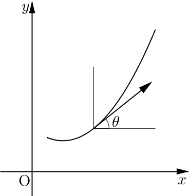
[Theorem 0.4]
평면 곡선 \(\mathbf x=\mathbf x(s)\)의 단위 접벡터 \(\mathbf t\)에 대하여 벡터 \(\mathbf t\)가 \(x\)축의 양의 방향과 이루는 각의 크기를 \(\theta\)라고 하자. 그러면 상수 \(C_1, \ C_2\)에 대하여 \[\begin{align} &\theta=\int\kappa ds+C_1 \\[.3em] &\mathbf x=\int (\cos\theta, \, \sin\theta)ds+C_2=\int \frac{1}{\kappa(\theta)}(\cos\theta, \,\sin\theta)d\theta+C_2\end{align}\]이다.
# 증명 ▶
(Proof)
\(\theta\)의 정의에 의하여 \(\mathbf t=(\cos \theta, \, \sin\theta)\)이고, 평면곡선에서는 \(\mathbf n\)이 \(\mathbf t\)를 시계 반대방향으로 90도 회전시킨 벡터이므로 \(\mathbf n=(-\sin\theta, \, \cos\theta)\)로 주어진다. 이 두 등식의 양변을 미분하면 \[\begin{align} &\mathbf{\dot t}=\dot{\theta}(-\sin\theta, \, \cos\theta)=\dot{\theta}\mathbf n\\[.3em] &\mathbf {\dot n}=\dot{\theta}(-\cos\theta, \, -\sin\theta)=-\dot{\theta}\mathbf t \end{align}\]이고, 프레네 - 세레 공식에 의하여 \(\mathbf {\dot t}=\kappa \mathbf n, \; \mathbf {\dot n}=-\kappa \mathbf t\)이므로 이 미분방정식의 해가 존재하기 위한 필요충분조건은 \(\dot {\theta}=\kappa\)이다. 따라서 \(\theta=\int \kappa ds+C_1\, \)이다. 이때 치환적분법을 이용하면 \[\begin{align}\mathbf x&=\int \mathbf tds+C_2 \\[.4em]&=\int(\cos\theta, \, \sin\theta)ds+C_2 \\[.4em] &=\int \left[(\cos\theta,\, \sin\theta)\cdot \frac{ds}{d\theta}\right]d\theta+C_2 \\[.4em]&= \int \frac{1}{\kappa(\theta)}(\cos\theta, \, \sin\theta)\,d\theta+C_2 \end{align}\]을 얻는다.
# ◀ 닫기
[Example 0.5]
내재적 방정식 \(\kappa=1/s\), \(\tau=0\), \(s>0\)를 만족시키는 곡선을 \(\mathbf x\)라고 하자. 이때 \(\dot{\theta}=\kappa=1/s\)이므로 \(\theta=\log s+C_1=\log(1/\kappa)+C_1\)이다. 이를 이용하면 \(\kappa=e^{-\theta+C_1}\)이다. 따라서 \[\begin{align} \mathbf x&=\int\frac{1}{\kappa}(\cos\theta, \, \sin\theta)d\theta\\[.3em]&=\int e^{\theta-C_1}(\cos\theta, \, \sin\theta)d\theta \\[.3em]&=\frac{1}{2}e^{\theta-C_1}(\cos\theta+\sin\theta, \, \sin\theta-\cos\theta)+C_2\\[.5em] &\stackrel{C_1=\frac{\pi}{4}, \ C_2=0}=\frac{1}{\sqrt{2}}e^{\theta-\frac{\pi}{4}}(\cos(\theta-\pi/4), \, \sin(\theta-\pi/4))\\[.3em]&\stackrel{\theta-\frac{\pi}{4}=\phi}=\frac{1}{\sqrt{2}}\,e^{\phi}(\cos\phi, \, \sin\phi) \end{align}\] 이다. 이는 다음과 같이 극형식으로 나타낼 수도 있다. \[r=\frac{1}{\sqrt{2}}e^\phi\]
여러 가지 문제들
[Problem 1.0]
다음 방정식으로 주어진 현수선(catenary)의 내재적 방정식을 구하시오. \[\mathbf x=(a\cosh(t/a), \ t), \quad a=\text{constant}\]
# 증명 ▶
(Proof)
주어진 도형은 평면 곡선이므로 \(\tau=0\)이다. 이때 \[\mathbf x'=(\sinh(t/a), \ 1), \ \ |\mathbf x'|=\sqrt{\sinh^2(t/a)+1}=\cosh(t/a)\]이므로 \[s=\int_0^t |\mathbf x'|dt=a\sinh(t/a) \; \Rightarrow \; \cosh^2(t/a)=\frac{s^2+a^2}{a^2}\]이다. 또한 \(\mathbf x''=(\frac{1}{a}\cosh(t/a), \, 0)\)이다. 따라서 \[\begin{align}\kappa&=\frac{\det(\mathbf x' \, \mathbf x'')}{|\mathbf x'|^3}\\[.4em]&=\frac{-1/a\cosh(t/a)}{\cosh^3(t/a)}\\[.4em]&=-\frac{1}{a\cosh^2(t/a)}=-\frac{a}{s^2+a^2}\end{align}\]이다.
# ◀ 닫기
[Problem 1.1]
반지름이 \(a\)인 구 위에 \(\tau\neq 0\)인 곡선이 있다. 이때 다음을 보이시오.
\[\mathbf{(a)} \ \ \displaystyle \left(\frac{1}{\kappa}\right)^2+\left(\frac{\dot \kappa}{\kappa^2\tau}\right)^2=a^2, \quad \mathbf{(b)}\ \ \displaystyle \frac{d}{ds}\left(\frac{\dot \kappa}{\kappa^2\tau}\right)=\frac{\tau}{\kappa}\]
# 증명 ▶
(Proof)
(a) 구의 중심을 \(\mathbf {x_0}\)라고 하자. 그러면 \((\mathbf{x-x_0})\cdot(\mathbf{x-x_0})=a^2\, \)이다. 이 등식의 양변을 미분하면 \[\mathbf {\dot x}\cdot (\mathbf{x-x_0})=0 \ \Rightarrow \ \mathbf t\cdot (\mathbf{x-x_0})=0\]이다. 다시 이 등식의 양변을 미분하면 \[\mathbf {\dot t}\cdot (\mathbf{x-x_0})+\mathbf t\cdot \mathbf t=0 \ \Rightarrow \ \mathbf n\cdot (\mathbf{x-x_0})=-\frac{1}{\kappa}\]이다. 이 등식의 양변을 다시 미분하면 \[\begin{align} &\mathbf {\dot n}\cdot (\mathbf{x-x_0})+\mathbf {n\cdot \dot{x}}=\frac{\dot \kappa}{\kappa^2}\\[.2em] & \Rightarrow \ (-\kappa\mathbf t+\tau \mathbf b)\cdot (\mathbf{x-x_0})=\frac{\dot \kappa}{\kappa^2}\\[.2em] & \Rightarrow \ \mathbf b\cdot (\mathbf{x-x_0})=\frac{\dot \kappa}{\kappa^2\tau} \end{align}\] 이때 \(\mathbf {t, \, n, \, b}\)가 정규직교기저를 이루므로 \[\mathbf {x-x_0}=-\frac{1}{\kappa}\mathbf n+\frac{\dot \kappa}{\kappa^2\tau}\mathbf b\]이고, \[(\mathbf{x-x_0})\cdot(\mathbf{x-x_0})=\left(\frac{1}{\kappa}\right)^2+\left(\frac{\dot \kappa}{\kappa^2\tau}\right)^2=a^2 \]이다.
(b) (a)에서 \(\mathbf {b\cdot (x-x_0)}=\displaystyle \frac{\dot \kappa}{\kappa^2\tau}\,\)이다. 이 등식의 양변을 미분하면 \[\begin{align}&\mathbf{\dot b}\cdot (\mathbf{x-x_0})+\mathbf b\cdot \mathbf {\dot x}=\frac{d}{ds}\left(\frac{\dot \kappa}{\kappa^2\tau}\right)\\[.5em] &\Rightarrow -\tau\mathbf n\cdot (\mathbf {x-x_0})=\frac{\tau}{\kappa}=\frac{d}{ds}\left(\frac{\dot \kappa}{\kappa^2\tau}\right)\end{align}\]을 얻는다.
# ◀ 닫기
[Problem 1.2]
곡선 \(C\)의 열률 \(\tau\)가 상수일 필요충분조건은 곡선 \(C\)의 방정식 \(\mathbf x\)가 \(0\)이 아닌 상수 \(a\)와 \(|g(t)|=1, \; \det(g \, g' \, g'')\neq 0\)을 만족시키는 벡터 함수 \(g(t)\)에 대하여 \[\mathbf x=a\int g(t)\times g'(t)\, dt\]로 나타낼 수 있는 것임을 보여라.
# 증명 ▶
(Proof)
(\(\Rightarrow\)) \(\tau=1/a\)라 하자. 그러면 \[\begin{align}&\mathbf {\dot b}=-\tau \mathbf n=-\frac{1}{a}\mathbf n \\[.4em] &\Rightarrow \mathbf {b\times \dot b}=-\frac{1}{a}(\mathbf {b\times n})=\frac{1}{a}\mathbf t \end{align}\] 따라서 \(\mathbf b=g\)라 하면 \(|g|=1\)이고, \[\mathbf {\ddot b}=-\frac{1}{a}\mathbf {\dot n}=-\frac{1}{a}(-\kappa \mathbf t+\tau \mathbf b)\]이므로 \(\det(g, \, g', \, g'')=\kappa/a^2\neq 0\)이다. 또한 \[\mathbf x=a\int \mathbf tds=a\int (g\times g')ds\]이다.
(\(\Leftarrow\)) \(\mathbf x=a\int g(t)\times g'(t)dt, \; |g(t)|=1, \; \det(g, \, g', \, g'')\neq 0\)이라 하자. 계산에 의하여 \[\begin{align}&\mathbf x'=a(g\times g')\\[.4em] &\mathbf x''=a(g'
\times g'+g\times g'')=a(g\times g'') \\[.4em] &\mathbf x'
''=a(g'\times g''+g\times g''')\end{align}\]이고 이로부터 \[\begin{align}\mathbf x'\times \mathbf x''&=a^2[\det(g \ g \ g'')\,g'-\det(g' \ g \ g'')\, g]\\[.4em]&=a^2\det(g \ g' \ g'')\, g\end{align}\]를 얻는다. 따라서 \[\begin{align}\tau&=\frac{\det(\mathbf x' \ \mathbf x'' \ \mathbf x''')}{|\mathbf x'\times\mathbf x''|^2}\\[.5em]&=\frac{(\mathbf x'\times\mathbf x'')\cdot \mathbf x'''}{a^4|\det(g \ g' \ g'')|^2|g|^2}\\[.5em]&=\frac{a^3\det(g \ g' \ g'')\, g\cdot(g'\times g''+g\times g''')}{a^4(\det(g \ g' \ g''))^2}\\[.5em] &=\frac{a^3 (\det (g \ g' \ g''))^2}{a^4(\det (g \ g' \ g''))^2}=\frac{1}{a}\end{align}\]이다.
# ◀ 닫기
[Problem 1.3]
두 곡선 \(C\)와 \(C^*\)가 대응되는 각 점에서 주법선이 동일하면, 두 곡선을 '버트란드 곡선(Bertrand Curves)'라고 한다. 이때 다음을 보이시오.
(a) 두 곡선 \(C\)와 \(C^*\)의 대응되는 각 점 사이의 거리는 일정하다.
(b) 두 곡선 \(C\)와 \(C^*\)의 대응되는 각 점에서의 접선이 이루는 각이 일정하다.
(c) 곡선 \(C\)의 각 점에서 열률이 \(0\)이 아닐 때, \(C\)가 버트란드 곡선이 되는 (즉, 곡선 \(C^*\)가 존재하여 두 곡선 \(C, \, C^*\)가 버트란드 곡선이 되는) 필요충분조건은 두 상수 \(\alpha, \, \gamma\)가 존재하여 \(\kappa+\gamma \tau =1/\alpha\)를 만족시키는 것임을 보여라.
# 증명 ▶
(Proof)
(a) 두 곡선 \(C\)와 \(C^*\)의 방정식이 각각 \(\mathbf x=\mathbf x(s)\), \(\mathbf x^*=\mathbf x^*(s)\)으로 주어졌다고 하자. \(C\)와 \(C^*\)에서의 각 점에서 주법선이 일치하므로 실함수 \(\alpha\)에 대하여 \(\mathbf x-\mathbf x^*=\alpha(s)\mathbf n(s)\)이 성립한다. 양변을 \(s\)에 대해 미분하면 \[\begin{align}\frac{d\mathbf x^*}{ds}&=\mathbf {\dot x}+\dot \alpha\mathbf n+\alpha\mathbf {\dot n}\\[.4em]&=\mathbf t+\dot \alpha\mathbf n+\alpha(-\kappa\mathbf t+\tau \mathbf b)\\[.4em] &=(1-\kappa\alpha)\mathbf t+\dot{\alpha}\mathbf n+\alpha\tau\mathbf b\end{align}\]을 얻는다. 이때 버트란드 곡선의 정의로부터 \(\displaystyle \frac{d\mathbf x^*}{ds}\)는 \(\mathbf n\)과 수직이므로 \[\{(1-\kappa\alpha)\mathbf t+\dot{\alpha}\mathbf n+\alpha\tau\mathbf b\}\cdot \mathbf n=\dot \alpha=0\]이다. 따라서 \(\alpha\)는 상수이고, \[|\mathbf {x^*-x}|=|\alpha \mathbf n|=|\alpha|=(\text{constant})\]
(b) 두 곡선 \(C\)와 \(C^*\)의 단위 접벡터를 각각 \(\mathbf t, \, \mathbf t^*\)라 하자. 그러면 \(\mathbf t\cdot \mathbf t^*\)의 값이 상수임을 보이면 충분하다. 이때 두 곡선의 주법선은 동일하므로 \[\begin{align}\frac{d}{ds}(\mathbf t\cdot \mathbf t^*)&=\mathbf {\dot t}\cdot \mathbf t^*+\mathbf t\cdot \dot{\mathbf{t^*}}\\[.1em]&=\kappa(\mathbf n\cdot \mathbf t^*)+\kappa^*(\mathbf t\cdot \mathbf n^*)=0\end{align}\]이다. 따라서 \(\mathbf t\cdot \mathbf t^*\)의 값은 상수이고, 두 곡선이 대응되는 각 점에서 접선이 이루는 각의 크기는 일정하다.
(c) (\(\Rightarrow\)) (a)에 의하여 상수 \(\alpha\)에 대하여 버트란드 곡선 \(C\)와 \(C^*\)의 방정식 \(\mathbf x,\, \mathbf x^*\)에 대하여 \(\mathbf x^*=\mathbf x+\alpha \mathbf n\)이 성립한다. (a), (b)의 결론으로부터 상수 \(\beta\)에 대하여 \[\begin{align}&\frac{d\mathbf x^*}{ds}=\dot{\mathbf t^*}\cdot \frac{ds^*}{ds}=(1-\alpha\kappa)\mathbf t+\alpha\tau\mathbf b\\[.2em] &\Rightarrow \, \mathbf t\cdot \dot {\mathbf t^*}=(1-\alpha\kappa)\cdot\frac{ds}{ds^*}=\cos\beta \quad \cdots \ (1) \end{align}\]이고, \(\mathbf t^*\)은 \(\mathbf t\)와 \(\mathbf b\)가 이루는 평면 위에 있으므로 \[\mathbf {b\cdot t^*}=\alpha\tau \frac{ds}{ds^*}=\pm \sin\beta \quad \cdots \ (2)\]이다. \((1), (2)\)에서 \(ds/ds^*\)를 소거하고 정리하면 \[\kappa\pm \tau \cot \beta =1/\alpha \; \Rightarrow \; \kappa+\gamma \tau =1/\alpha \; (\gamma=\pm \cot \beta)\]을 얻는다.
(\(\Leftarrow\)) 곡선 \(C\)가 가정을 만족시킨다고 하고, 곡선 \(C^*\)를 \(\mathbf x^*=\mathbf x+\alpha\mathbf n\, \)이라고 정의하자. 그러면 \[\frac{d\mathbf x^*}{ds}=(1-\alpha\kappa)\mathbf t+\alpha\tau\mathbf b=\alpha\tau (\gamma\mathbf t+\mathbf b)\]이다. 이로부터 \[\left|\frac{d\mathbf x^*}{ds}\right|=|\alpha\tau|\sqrt{\gamma^2+1} \; \Rightarrow \; \mathbf t^*=\frac{d\mathbf x^*}{ds}/\left|\frac{d\mathbf x^*}{ds}\right|=\pm\frac{\gamma\mathbf t+\mathbf b}{\sqrt{\gamma^2+1}}\]이다. 따라서 \[\begin{align}&\frac{d\mathbf t^*}{ds}=\pm\frac{\gamma\mathbf {\dot t}+\mathbf {\dot b}}{\sqrt{\gamma^2+1}}=\pm\frac{\gamma\kappa-\tau}{\sqrt{\gamma^2+1}}\mathbf n \\[.5em] \end{align}\]이므로 \(\mathbf n\)과 \(\mathbf n^*\)은 평행하다. 즉, \(\mathbf n=\pm \mathbf n^*\)이다. 따라서 두 곡선은 버트란드 곡선이다.
# ◀ 닫기
Reference: <Schaum's Outlines: Differential Geometry> Martin Lipschultz, 1969
'[Undergraduates] > 미분기하학' 카테고리의 다른 글
| [Chapter 8] Concept of a Surface - (2) (0) | 2021.05.24 |
|---|---|
| [Chapter 8] Concept of a Surface - (1) (0) | 2021.05.12 |
| [Chapter 3~4] Concept of Curve + Curvature and Torsion (0) | 2021.04.24 |